CyberShake BBP Integration
This page details the process of integrating CyberShake with the Broadband Platform, so that we can produce stochastic high-frequency seismograms in CyberShake as a complement to deterministic low-frequency seismograms.
We performed a similar integration process for CyberShake 1.4 and CyberShake Study 15.12. This time, we would like to avoid maintaining a separate CyberShake version of the high-frequency stochastic codes. Instead, we would like to invoke the BBP codes from CyberShake, so that as new modifications are made to BBP, CyberShake can use these new codes without requiring the entire integration process again.
Contents
Approach
We have identified the following BBP executables, or elements, which are needed in CyberShake:
- srf2stoch (C)
- hb_high (Fortran)
- wcc_getpeak (C)
- wcc_siteamp14 (C)
- wcc_tfilter (C)
- wcc_resamp_arbdt (C)
- wcc_add (C)
- integ_diff (C)
As part of the BBP, each of these pieces of code contains a main() function, which typically works as follows:
main() {
  // Parse command-line parameters
  // Open and read input files into input data structure
  // Execute science kernel, populating output data structure
  // Open and write output files from output data structure
}
For CyberShake, we would like to be able to use the science kernels of the BBP elements, but provide CyberShake-specific parameters, pass data structures around in memory between multiple elements, and read from and write to different data formats. To accomplish this, we propose extracting the science kernels from the main() functions and creating subroutines with them, separating the I/O from the scientific calculations. Following this approach, a revised main method would contain:
main() {
  // Open and read input files into input data structure
  science_kernel_subroutine(command-line arguments, input_data_structure, output_data_structure)
  // Open and write output files from output data structure
}

science_kernel_subroutine(command-line arguments, input_data_structure, output_data_structure) {
  // Use input data structure for processing
  // Place results in output data structure
}
Then, in the CyberShake codebase, we would use this function as follows:
// Open and read input files into input data structure
// Allocate memory for output data structure
// Create parameter string with CyberShake-specific parameters for getpar to parse
science_kernel_subroutine(parameter_string, input_data_structure, output_data_structure)
// Do additional processing with output data structure
// Open and write output data structure to file
The intent is that these changes would be pushed out to the BBP codebase and also to Rob Graves, so that future revisions work from this refactored version and are straightforward to integrate with CyberShake.
Filename convention
Since for CyberShake we link the CyberShake code with the subroutine object files, the BBP main methods can't be in the subroutine object files (otherwise we would have multiple main()s), and must be contained in separate files. The convention we will follow is to have all subroutines in <module>_sub.c, and the main method with subroutine prototypes in <module>_main.c. The compiled executable used by BBP will have the name <module>_sub, to distinguish it from the non-refactored executables when testing.
Example
As an example, below we show the proposed modifications for wcc_getpeak. wcc_getpeak doesn't have an output data structure; in the BBP the result is printed, whereas in the subroutine it is returned.
| Change | Original code | Modified code |
|---|---|---|
| Subroutine prototype | N/A | float wcc_getpeak(int param_string_len, char** param_string, float* seis, struct statdata* head1); |
| Extract science kernel into subroutine |
int main(ac,av) { |
... |
| Relocate parsing of non-I/O parameters to subroutine | int main(ac,av) { |
float wcc_getpeak(int param_string_len, char** param_string, float* s1, struct statdata* head1) { |
| Retain I/O in main function |
int main(ac,av) |
int main(ac,av) |
Here is a way CyberShake code could use this modified code:
...
float* seis = malloc(nt*sizeof(float));
fread(fp_in, sizeof(float), nt, seis);
struct statdata head1;
head1.nt = nt;
char** param_string = NULL;
float peak = wcc_getpeak(param_string, 0, seis, &head1);
...
Migration Status
| Element | Refactored | Passes BBP test | Called from CyberShake |
|---|---|---|---|
| wcc_getpeak | yes | yes | |
| wcc_add | yes | yes | |
| wcc_tfilter | yes | yes | |
| wcc_resamp_arbdt | yes | yes | |
| integ_diff | yes | yes | |
| wcc_siteamp14 | yes | yes | |
| hb_high | yes | yes | yes |
| srf2stoch | yes | yes | yes |
Verification
hb_high
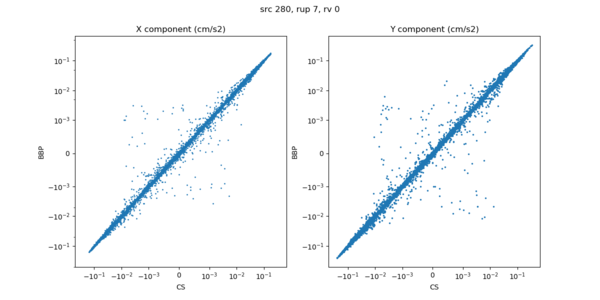
hb_high is the most difficult code to verify, as it's the most complex.
To assist in verification, we constructed scatter plots comparing the value in CyberShake-calling-BBP to the value in BBP directly, for each point in the acceleration time series.
Our initial results are

|
Upon further investigation, we uncovered a few issues.
- The default value in the BBP for kappa is 0.04, which is what we are using in CyberShake. However, when using the LA Basin velocity model, the default value is overwritten in the BBP and 0.045 is used instead. Once we updated to the right value of kappa, that improved the scatter a bit:
- In the CyberShake code, the geographic coordinates are rounded to 4 decimal places to agree with the output file that srf2stoch produces. However, this rounding is accomplished by multiplying, adding 0.5, casting to an int as a floor(), and then dividing. This is fine for positive numbers, but for negative numbers int and floor are not equivalent. Casting to an int will truncate towards 0, and floor() will truncate towards negative infinity. The rounding used when C writes files matches using floor().
Once this modification is also made, the seismograms very closely agree:
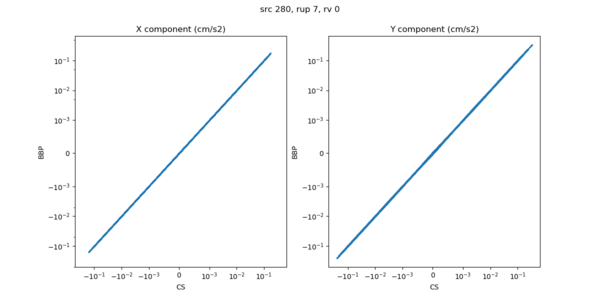


A visual comparison looks good:

A numerical comparison is also good:
Average absolute difference: 0.000000
Max absolute difference: 0.000005
Average absolute percent difference: 0.024559
Max absolute percent difference: 150.758352
Bins:
0.000000 <= reference amplitude < 0.010000:
	avg diff=0.000000, avg percent diff=0.028306%
0.010000 <= reference amplitude < 0.100000:
	avg diff=0.000000, avg percent diff=0.000988%
0.100000 <= reference amplitude < 1.000000:
	avg diff=0.000002, avg percent diff=0.001870%
1.000000 <= reference amplitude < 10.000000:
Site Response
Visual comparisons for source 280, rupture 7, rv 0:

|

|

|
The scatterplot:

|
A numerical comparison looks good:
Average absolute difference: 0.000004
Max absolute difference: 0.000069
Average absolute percent difference: 0.265180
Max absolute percent difference: 265.281916
Bins:
0.000000 <= reference amplitude < 0.010000:
	avg diff=0.000001, avg percent diff=0.297034%
0.010000 <= reference amplitude < 0.100000:
	avg diff=0.000022, avg percent diff=0.076535%
0.100000 <= reference amplitude < 1.000000:
1.000000 <= reference amplitude < 10.000000:
10.000000 <= reference amplitude < 100.000000:
100.000000 <= reference amplitude < 1000.000000:
1000.000000 <= reference amplitude < 10000.000000:
Filtered comparisons
Comparisons should be done using filtered seismograms (2-pass 4th order Butterworth, high-pass at 1 Hz). Below are results for all 10 ruptures after filtering. Each rupture has approximately 60% more rupture surface points than the previous rupture.
The differences in scatter starting with the Garlock rupture can be traced to differences in a division followed by a floor().
For example, a value in the rupt array (which I think is initiation time) is 2.64000e+01. In the CyberShake code, this is represented by 26.3999691; in the BBP code, 26.3999996. The input dt is set to 0.01, but that is represented as 9.99999978E-03. The rupt value divided by dt gives 2639.99707 for CyberShake and 2640.00000 for BBP. Taking the floor, then, gives 2639 for CyberShake and 2640 for BBP. This value is used as an offset into an array, which is then multiplied by another value, so the difference is magnified. Compiling with O0 does not reduce the error.
We seem to get larger/more differences for events with larger ground motions.
| Event | Seismogram | Zoomed Seismogram | Scatterplot | Numerical comparison |
|---|---|---|---|---|
| Source 280 Rupture 7 Rup var 0 Tank Canyon, M6.65 |

|

|

|
12093 of 100000 values above threshold 1e-06 Average absolute difference: 0.000001 Max absolute difference: 0.000012 Average absolute percent difference: 1.488839 Max absolute percent difference: 26.480208 Bins: 1.0e-06 <= reference amplitude < 0.01: avg diff=0.000001, avg % diff=1.43% 0.01 <= reference amplitude < 0.1: avg diff=0.000007, avg % diff=0.0507% 0.1 <= reference amplitude < 1.0: None |
| Source 269 Rupture 8 Rup var 1 Santa Monica, M6.85 |

|

|

|
49372 of 100000 values above threshold 1e-06 Average absolute difference: 0.000016 Max absolute difference: 0.001929 Average absolute percent difference: 5.249444 Max absolute percent difference: 210.588523 Bins: 1.0e-06 <= reference amplitude < 0.01: avg diff=0.000001, avg % diff=5.46% 0.01 <= reference amplitude < 0.10: avg diff=0.000166, avg % diff=0.381% 0.10 <= reference amplitude < 1.00: avg diff=0.000698, avg % diff=0.334% 1.00 <= reference amplitude < 10.00: None |
| Source 220 Rupture 10 Rup var 2 North Channel, M6.85 |

|

|

|
49686 of 100000 values above threshold 1e-06 Average absolute difference: 0.000002 Max absolute difference: 0.000124 Average absolute percent difference: 2.517283 Max absolute percent difference: 25.023028 Bins: 1.0e-06 <= reference amplitude < 0.01: avg diff=0.000000, avg % diff=2.71% 0.01 <= reference amplitude < 0.10: avg diff=0.000018, avg % diff=0.0608% 0.10 <= reference amplitude < 1.00: avg diff=0.000080, avg % diff=0.0667% 1.00 <= reference amplitude < 10.00: None |
| Source 269 Rupture 24 Rup var 3 Santa Ynez, M6.95 |

|

|

|
49313 of 100000 above threshold 1e-06 Average absolute difference: 0.000001 Max absolute difference: 0.000062 Average absolute percent difference: 6.031340 Max absolute percent difference: 18.205049 Bins: 1.0e-06 <= reference amplitude < 0.01: avg diff=0.000000, avg percent diff=6.32% 0.01 <= reference amplitude < 0.10: avg diff=0.000015, avg percent diff=0.0606% 0.10 <= reference amplitude < 1.00: avg diff=0.000061, avg percent diff=0.0578% 1.00 <= reference amplitude < 10.00: None |
| Source 105 Rupture 3 Rup var 4 San Jacinto, M6.95 |

|

|

|
16886 of 100000 values above threshold 1e-06 Average absolute difference: 0.000001 Max absolute difference: 0.000019 Average absolute percent difference: 0.202181 Max absolute percent difference: 19.772487 Bins: 1.0e-06 <= reference amplitude < 0.01: avg diff=0.000001, avg % diff=0.210% 0.01 <= reference amplitude < 0.10: avg diff=0.000009, avg % diff=0.0584% 0.10 <= reference amplitude < 1.00: None |
| Source 21 Rupture 2 Rup var 5 Garlock, M7.15 |

|

|

|
49823 of 100000 values above threshold 1e-06 Average absolute difference: 0.000031 Max absolute difference: 0.002349 Average absolute percent difference: 6.556178 Max absolute percent difference: 68462.868722 Bins: 1.0e-06 <= reference amplitude < 0.01: avg diff=0.000008, avg % diff=7.18% 0.01 <= reference amplitude < 0.10: avg diff=0.000238, avg % diff=0.961% 0.10 <= reference amplitude < 1.00: avg diff=0.000484, avg % diff=0.449% 1.00 <= reference amplitude < 10.00: None |
| Source 100 Rupture 1 Rup var 6 San Jacinto, M7.25 |

|

|

|
48228 of 100000 values above threshold 1e-06 Average absolute difference: 0.000019 Max absolute difference: 0.000873 Average absolute percent difference: 21.214481 Max absolute percent difference: 2036.818780 Bins: 1.0e-06 <= reference amplitude < 0.01: avg diff=0.000005, avg % diff=24.45% 0.01 <= reference amplitude < 0.10: avg diff=0.000095, avg % diff=0.298% 0.10 <= reference amplitude < 1.00: avg diff=0.000227, avg % diff=0.162% 1.00 <= reference amplitude < 10.00: None |
| Source 10 Rupture 1 Rup var 7 Elsinore, M7.55 |

|

|

|
49416 of 100000 values above threshold 1e-06 Average absolute difference: 0.000274 Max absolute difference: 0.018217 Average absolute percent difference: 11.981339 Max absolute percent difference: 12207.828835 Bins: 1.0e-06 <= reference amplitude < 0.01: avg diff=0.000019, avg % diff=15.68% 0.01 <= reference amplitude < 0.10: avg diff=0.000608, avg % diff=1.714% 0.10 <= reference amplitude < 1.00: avg diff=0.001434, avg % diff=0.625% 1.00 <= reference amplitude < 10.00: avg diff=0.000409, avg % diff=0.0349% 10.00 <= reference amplitude < 100.00: None |
| Source 86 Rupture 0 Rup var 8 San Andreas, M7.65 |

|

|

|
50394 of 100000 values above threshold 1.000000e-06 Average absolute difference: 0.002977 Max absolute difference: 0.098694 Average absolute percent difference: 15.380488 Max absolute percent difference: 32075.901501 Bins: 1.0e-06 <= reference amplitude < 0.01: avg diff=0.000096, avg % diff=22.57% 0.01 <= reference amplitude < 0.10: avg diff=0.003266, avg % diff=8.784% 0.10 <= reference amplitude < 1.00: avg diff=0.008658, avg % diff=2.653% 1.00 <= reference amplitude < 10.00: avg diff=0.010934, avg % diff=0.799% 10.00 <= reference amplitude < 100.00: None |
| Source 128 Rupture 1296 Rup var 9 San Andreas, M8.45 |

|

|

|
64646 of 100000 values above threshold 1.000000e-06 Average absolute difference: 0.006450 Max absolute difference: 0.206112 Average absolute percent difference: 19.995406 Max absolute percent difference: 163277.921485 Bins: 1.0e-06 <= reference amplitude < 0.01: avg diff=0.000113, avg % diff=31.06% 0.01 <= reference amplitude < 0.10: avg diff=0.005178, avg % diff=13.34% 0.10 <= reference amplitude < 1.00: avg diff=0.016088, avg % diff=4.456% 1.00 <= reference amplitude < 10.00: avg diff=0.019644, avg % diff=1.262% 10.00 <= reference amplitude < 100.00: None |
Low-frequency site response
We performed low-frequency site response comparisons using the same set of ruptures. This resulted in an average absolute difference of ~2e-5. In all but the smallest value bin, percent differences are between 0.05 and 0.0002%. These results are several orders of magnitude closer than the high-frequency results, and are close enough for our purposes.
Merging code
The merging code low-pass filters the low-frequency seismogram (after site response has been added), resamples it at the same dt as the high frequency seismogram, combines the two, and then processes to obtain IM values. We ran our tests using the standard set of rupture variations and found that the average absolute difference was around 1e-6. In all but the smallest value bin, percent differences are less than 0.005%. These results are better than either the high-frequency or site response results, and are good enough for our purposes.
Changes from Study 15.12
We pioneered the general concept of performing stochastic calculations alongside deterministic ones in CyberShake_1.4 and then futher developed it in CyberShake_Study_15.12. For this integration effort, we are going to make a few changes from the Study 15.12 work.
- Since the low-frequency content of the stochastic seismograms should be ignored, we are moving the HF filtering from the MergeIM step into HFSim so that we aren't tempted to use the stochastic output of that code unfiltered.
- We have decided to low-pass filter the deterministic seismograms before merging. This will be done in the MergeIM stage.
Results
Spot tests
Below are example seismograms from each step of the process (deterministic, deterministic + site response, stochastic, and merged) for 4 different ruptures.
| Event | Deterministic | Deterministic + site response | Stochastic | Merged |
|---|---|---|---|---|
| Santa Ynez M6.95 s269 r24 rv3 |

|

|

|

|
| Garlock M7.15 s21 r2 rv5 |

|

|

|

|
| Elsinore M7.55 s10 r1 rv7 |

|

|

|

|
| S. San Andreas M8.15 s128 r1296 rv9 |

|

|

|

|
TEST site
The below results were obtained from running the TEST site.
| 10 sec | 5 sec | 3 sec | 2 sec |
|---|---|---|---|


| 1 sec | 0.5 sec | 0.2 sec | 0.1 sec |
|---|---|---|---|


Below are seismograms for 4 events: small (M6.55) and large (M7.35) close (<= 6 km) and far (>=19 km). Once we run a full site we can test events much farther away.
| Event | Deterministic seismogram | Broadband seismogram |
|---|---|---|
| Puente Hills, M6.55 (2.5km) src 244, rup 5, rv 44 |
||
| Puente Hills, M7.35 (5.7km) src 242, rup 29, rv 62 |
||
| Newport-Inglewood, M6.55 (19.7km) src 216, rup 4, rv 9 |
||
| Newport-Inglewood, M7.35 (19.2 km) src 218, rup 251, rv 10 |
||


USC
Below are seismograms for 4 events: small and large, close and far.
| Event | Deterministic seismogram | Broadband seismogram |
|---|---|---|
| Santa Monica, M7.05 (12.9km) src 264, rup 79, rv 109 |
||
| Newport Inglewood, M7.75 (7.0km) src 219, rup 267, rv 73 |
||
| San Andreas BG+CO, M7.05 (137.1km) src 51, rup 0, rv 130 |
||
| So. Sierra Nevada, M7.75 (143.8km) src 276, rup 144, rv 125 |
||


Hazard Curves
Comparisons between new deterministic (Run 7130) and Study 15.4 (Run 3970) (change of rupture generator, hypocentral spacing)


Comparisons between new broadband (Run 7153) and Study 15.12 (Run 4384) (rupture generator, hypocentral spacing, BB codes)


Comparisons between new broadband (Run 7153) and new deterministic (Run 7130) (site response)


