Seismtools
This page describes the seismogram processing package called Seismtools, originally created by Ricardo Taborda's research group at the University of Memphis. This package was forked from its original location at ASEIS/seismtools and developed at SCEC's SCECcode/seismtools GitHub repository. Modifications and improvements to the code are periodically contributed back to ASEIS' original repository. Here's a link to SCEC's forked seismtools repository:
Contents
Comparison of Python and Matlab Processing Results
SCECCode Seismtools
Below is a summary of the Seismtools package after a few SCEC modifications. Please refer to the section about ASEIS' Seismtools for information about the original software package from the ASEIS group. SCEC has modified the Seismtools package to add support for BBP files by including Hercules, AWP-ODC, and RWG to BBP migration tools so that other file formats can be converted to BBP format. Additionally, Seismtools can save processed files in BBP format. We have also extended the original tools so that users can work with multiple time series simultaneously (instead of just 1 observation and 1 synthetic). The current code allows for one observation and one (or more synthetics), or no observations and two (or more) synthetics to be compared. The plotting tools can take any number of time series. Below are the main steps required for using SCEC's Seismtools:
- Step 1A: process_smc.py
- Converts V2 files to BBP (or 10-column .her Hercules files)
- Rotates observation files to N/S, E/W, U/D if needed
- Outputs 3 BBP (or a single hercules) files in cm
- Usage: process_smc.py bbp <output_dir> <input_dir>
- Step 1B: her2bbp.py, awp2bbp.py, rwg2bbp.py
- Convert 10-col .her Hercules files, AWP-ODC files, or RWG .bbp files to BBP format
- Keep units from original files
- Hercules file split into 3 BBP files (dis, vel, acc)
- AWP/RWG velocity file goes through integration/derivation to create dis and acc files
- Metadata from RWG file is used to populate BBP header
- Users can provide metadata using command-line options (latitude/longitude/station name)
- Usage: her2bbp.py [-d <output_dir>] <input_file> <output_stem> [-s <station_name>]
- Step 2: process_timeseries.py
- Processes one observation file and one (or more) synthetics OR two or more synthetics
- Brings files to same DT
- Synthetics are assumed to be aligned and have the same orientation
- Observation time series and synthetics aligned using --eq-time and leading time
- Rotates synthetics by <rotation_angle> so that they are N/S, E/W, U/D
- Band pass filter using first and last frequencies in --bands parameter
- All time series converted to cm
- Outputs processed timeseries
- Usage: process_timeseries.py [--obs <observation_file>] timeseries_1 [timeseries_2 .. timeseries_n] --decimation_freq <n> --dt <new_dt> --azimuth <rotation angle> --eq_time <obs_time time> --leading <synthetics_lead_time>
- Step 3: simple_compare.py
- Plots velocity timeseries for the N/S, E/W, U/D components together with FAS plots and response spectra
- Usage: simple_compare.py N file1 <file2> .. <fileN> xmin xmax fmin fmax filter_flag [filter_min filter_max] rsp_min rsp_max cut_flag
Adding BBP File Format Compatibility
The seismtools package has been modified so that it is compatible with time series in BBP format. The process_smc.py script was modified so that the user is asked what format to output seismograms. In the case of the BBP file format, 3 BBP files are output for each input observation file (one containing each of displacement, velocity, and acceleration).
Here's a sample BBP file (shortened) produced by process_smc.py:
# Station: CI_FUL
#    time= 3/29/14,4:9:36.10 UTC
#     lon= 117.923W
#     lat= 33.872N
#   units= m/s
#
# Data fields are TAB-separated
# Column 1: Time (s)
# Column 2: N/S component ground velocity (+ is 000)
# Column 3: E/W component ground velocity (+ is 090)
# Column 4: U/D component ground velocity (+ is upward)
#
## Previous header is copied but each line prepended with another '#' character
## allowing keeping a history of processing stages
0.0000000   9.027200000e-03   -3.251600000e-03    -5.246600000e-03
0.0100000   9.067900000e-03   -3.256500000e-03    -5.257700000e-03
0.0200000   9.108600000e-03   -3.261100000e-03    -5.268600000e-03
0.0300000   9.149300000e-03   -3.265700000e-03    -5.279400000e-03
0.0400000   9.190000000e-03   -3.270200000e-03    -5.290200000e-03
0.0500000   9.230700000e-03   -3.274700000e-03    -5.300700000e-03
0.0600000   9.271600000e-03   -3.279000000e-03    -5.311200000e-03
Results 2016-07-22
The latest data sets include the following datasets:
- OBS
- RWG: There are results from 3 different sources, all using the small model region
- Point Source Model
- Finite-fault rupture model generated with GP 15.4
- Finite-fault rupture model from Shengji Wei
- SDSU
- Point Source in large 3D CVM region with new Vp/Vs clamping rules
- Hercules
- Small-domain
- Using damping and point source model
Processing steps:
- Observations and Synthetics are rotated to N/S, E/W
- All files brought to the same DT = 0.025
- Synchronized timeseries (observations, synthetics)
- Filtered observations and synthetics 4.0Hz
Data was filtered at 0.3Hz, 0.5Hz, 1.0Hz, 2.0Hz, and 4.0Hz.
- OBS + AWP + Hercules + RWG Point Source
- OBS + AWP + Hercules + RWG Finite Fault GP 15.4
- OBS + AWP + Hercules + RWG Finite Fault Shengi Wei
Validating 2016-03-21 Runs
We have used Seismtools to process the data set we had processed on March 21st, 2016. This data set includes synthetic time series from Hercules, RWG, and SDSU. Here are the plots along with plots using the original processing scripts:
- Processing steps
$ ./her2bbp.py -d /Users/fsilva/Work/git/highf/20160321/files/seismtools \
                  /Users/fsilva/Work/git/highf/20160321/files/hercules/station.5 CI_FUL-Hercules -s CI_FUL
$ ./her2bbp.py -d /Users/fsilva/Work/git/highf/20160321/files/seismtools \
                  /Users/fsilva/Work/git/highf/20160321/files/hercules/station.23 CI_BRE-Hercules -s CI_BRE
$ ./her2bbp.py -d /Users/fsilva/Work/git/highf/20160321/files/seismtools \
                  /Users/fsilva/Work/git/highf/20160321/files/hercules/station.41 CI_DLA-Hercules -s CI_DLA
$ ./awp2bbp.py -d /Users/fsilva/Work/git/highf/20160321/files/seismtools \
                  /Users/fsilva/Work/git/highf/20160321/files/small_corr_cerj90/CI_FUL.dat CI_FUL-AWP-ODP -s CI_FUL
$ ./awp2bbp.py -d /Users/fsilva/Work/git/highf/20160321/files/seismtools \
                  /Users/fsilva/Work/git/highf/20160321/files/small_corr_cerj90/CI_BRE.dat CI_BRE-AWP-ODP -s CI_BRE
$ ./awp2bbp.py -d /Users/fsilva/Work/git/highf/20160321/files/seismtools \
                  /Users/fsilva/Work/git/highf/20160321/files/small_corr_cerj90/CI_DLA.dat CI_DLA-AWP-ODP -s CI_DLA
$ ./rwg2bbp.py -d /Users/fsilva/Work/git/highf/20160321/files/seismtools \
                  /Users/fsilva/Work/git/highf/20160321/files/rwg/CI_FUL-RWG-vel.bbp CI_FUL-RWG
$ ./rwg2bbp.py -d /Users/fsilva/Work/git/highf/20160321/files/seismtools \
                  /Users/fsilva/Work/git/highf/20160321/files/rwg/CI_BRE-RWG-vel.bbp CI_BRE-RWG
$ ./rwg2bbp.py -d /Users/fsilva/Work/git/highf/20160321/files/seismtools \
                  /Users/fsilva/Work/git/highf/20160321/files/rwg/CI_DLA-RWG-vel.bbp CI_DLA-RWG
$ ./process_timeseries.py /Users/fsilva/Work/git/highf/20160321/files/seismtools/CI_FUL-RWG.vel.bbp \
                  /Users/fsilva/Work/git/highf/20160321/files/seismtools/CI_FUL-Hercules.vel.bbp \
                  /Users/fsilva/Work/git/highf/20160321/files/seismtools/CI_FUL-AWP-ODP.vel.bbp \
                  --output-dir /Users/fsilva/Work/git/highf/20160321/files/seismtools/process --bands "0.15 0.25 0.5 1 2 4" \
                  --decimation-freq 5 --dt 0.025 --azimuth 39.9 --eq-time 4:9:42.97 --leading 0
$ ./process_timeseries.py /Users/fsilva/Work/git/highf/20160321/files/seismtools/CI_BRE-RWG.vel.bbp \
                  /Users/fsilva/Work/git/highf/20160321/files/seismtools/CI_BRE-Hercules.vel.bbp \
                  /Users/fsilva/Work/git/highf/20160321/files/seismtools/CI_BRE-AWP-ODP.vel.bbp \
                  --output-dir /Users/fsilva/Work/git/highf/20160321/files/seismtools/process --bands "0.15 0.25 0.5 1 2 4" \
                  --decimation-freq 5 --dt 0.025 --azimuth 39.9 --eq-time 4:9:42.97 --leading 0
$ ./process_timeseries.py /Users/fsilva/Work/git/highf/20160321/files/seismtools/CI_DLA-RWG.vel.bbp \
                  /Users/fsilva/Work/git/highf/20160321/files/seismtools/CI_DLA-Hercules.vel.bbp \
                  /Users/fsilva/Work/git/highf/20160321/files/seismtools/CI_DLA-AWP-ODP.vel.bbp \
                  --output-dir /Users/fsilva/Work/git/highf/20160321/files/seismtools/process --bands "0.15 0.25 0.5 1 2 4" \
                  --decimation-freq 5 --dt 0.025 --azimuth 39.9 --eq-time 4:9:42.97 --leading 0
$ ./simple_compare.py 3 /Users/fsilva/Work/git/highf/20160321/files/seismtools/process/p-CI_FUL-RWG.vel.bbp \
                  /Users/fsilva/Work/git/highf/20160321/files/seismtools/process/p-CI_FUL-Hercules.vel.bbp \
                  /Users/fsilva/Work/git/highf/20160321/files/seismtools/process/p-CI_FUL-AWP-ODP.vel.bbp \
                  0 16 0 5 n 0 10 n
$ ./simple_compare.py 3 /Users/fsilva/Work/git/highf/20160321/files/seismtools/process/p-CI_BRE-RWG.vel.bbp \
                  /Users/fsilva/Work/git/highf/20160321/files/seismtools/process/p-CI_BRE-Hercules.vel.bbp \
                  /Users/fsilva/Work/git/highf/20160321/files/seismtools/process/p-CI_BRE-AWP-ODP.vel.bbp \
                  0 22 0 5 n 0 10 n
$ ./simple_compare.py 3 /Users/fsilva/Work/git/highf/20160321/files/seismtools/process/p-CI_DLA-RWG.vel.bbp \
                  /Users/fsilva/Work/git/highf/20160321/files/seismtools/process/p-CI_DLA-Hercules.vel.bbp \
                  /Users/fsilva/Work/git/highf/20160321/files/seismtools/process/p-CI_DLA-AWP-ODP.vel.bbp \
                  0 25 0 5 n 0 10 n
- Plots with new SCEC's Seismtools
- Plots using SCEC's old processing scripts (for comparison only)
- FUL - 040 component (Combined) (FFT), 130 component (Combined) (FFT), VER component (Combined) (FFT)
- BRE - 040 component (Combined) (FFT), 130 component (Combined) (FFT), VER component (Combined) (FFT)
- DLA - 040 component (Combined) (FFT), 130 component (Combined) (FFT), VER component (Combined) (FFT)
Original Seismtools package from ASEIS
Below is a brief description of some of the software components included in the seismtools repository:
- process_sdc.py - Processes Southern California Data Center ASCII files and generates Hercules format files
- process.py - Processes Strong Motion Center V1/V2 files and generates Hercules format files
- gof.py - Front end for producing GOF results, reads Hercules files, processes their signals, calculates scores and produces table
- gof_data_sim.py - Functions used by the gof.py script to process seismograms
- compare.py - Creates displacement, velocity, and acceleration comparison plots between two Hercules-formated files
- s_compare.py - Processes two Hercules files, and plots only velocity time series, FAS, and Response Spectra
- seism.py - Common structures (e.g. seismic record, station, etc)
- stools.py - Processing functions that can be used by other codes
Validating ASEIS Seismtools
The basic workflow for processing observation files and generating comparison plots is:
- Run process_sdc.py and/or process.py to convert seismograms to Hercules format
- Run gof.py code to process the observation and synthetic seismogram files, generating processed files and a table containing gof scores
- Run s_compare.py and/or compare.py to generate plots using the processed seismogram files generated by the gof.py stage above
Both processing observation seismograms scripts can be used to convert files to Hercules format in batch mode by taking a directory as input:
$ process_sdc.py /Users/shima/Desktop/Python_Steps/raw_data/ascii/
== Enter event ID (optional):
== Enter network code (optional):
== Enter station ID (optional):
== Enter sample rate and data type representation (optional):
== Enter name of the directory to store outputs: ascii
or
$ process.py  /Users/shima/Desktop/Python_Steps/raw_data/v/
== Enter name of the directory to store outputs: v
Then, users should run the gof.py tool in order to process the Hercules format seismograms and generate rotated/aligned/filtered seismograms:
$ gof.py /Users/shima/Desktop/Python_Steps/filelist
== Enter name of 1st input directory: /Users/shima/Desktop/Python_Steps/her
== Enter name of 2nd input directory: /Users/shima/Desktop/Python_Steps/sim
== Enter name of the directory to store outputs: /Users/shima/Desktop/Python_Steps/gof
== Enter name of scores file: scores.txt
== Enter name of matrics file: metrics.txt
== Enter the sequence of sample rates: 0.1 0.25 0.5 1
== Enter the maximum frequence for decimation: 2
== Enter common dt of two signals: 0.1
== Enter azimuth for rotation (optional): 39.9
== Enter the earthquake start time (#:#:#.#): 11:50:11.916
== Enter the simulation leading time (sec): 2
== Enter the X and Y coordinates of epicenter: 130962.750445 72713.652041
In case we want to run only two signals, we can use:
$ gof.py /Users/shima/Desktop/Python_Steps/her/CI.ALP.BH.her /Users/shima/Desktop/Python_Steps/sim/station.498
== Enter name of the directory to store outputs: out
== Enter name of scores file: scores.txt
== Enter name of matrics file: metrics.txt
== Enter the sequence of sample rates: 0.1 0.25 0.5 1
== Enter the maximum frequence for decimation: 2
== Enter common dt of two signals: 0.1
== Enter azimuth for rotation (optional): 39.9
== Enter the earthquake start time (#:#:#.#): 11:50:11.916
== Enter the simulation leading time (sec): 2
.....
Do you want to print the processed signals [y] or [n]: y
Once the processing stage is completed, users can generate plots using the following commands:
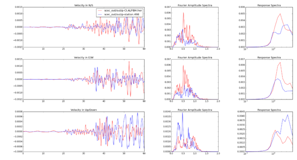
$ compare.py /Users/shima/Desktop/Python_Steps/out/p-CI.ALP.BH.her /Users/shima/Desktop/Python_Steps/out/p-station.498
== Enter T-min for ploting: 0
== Enter T-max for ploting: 60
== Enter F-min for ploting: 0
== Enter F-max for ploting: 2
== Do you want to filter the data (y/n): n
== Enter tmin for Response: 0
== Enter tmax for Response: 5
== Do you want to cut the signal (y/n): n
and:
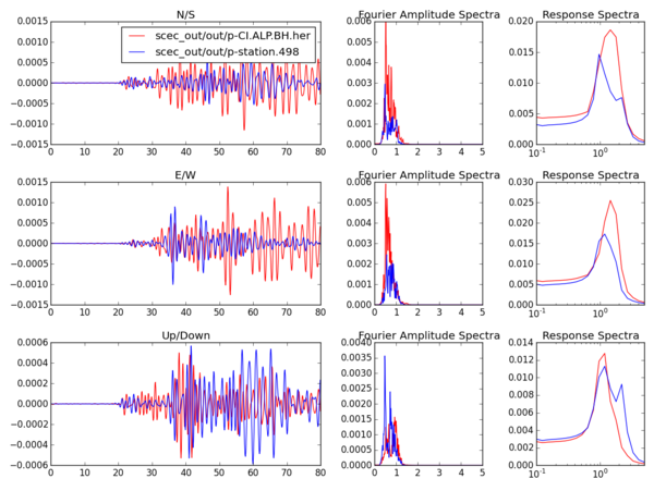
$ s_compare.py /Users/shima/Desktop/Python_Steps/out/p-CI.ALP.BH.her /Users/shima/Desktop/Python_Steps/out/p-station.498
== Enter T-min for ploting: 0
== Enter T-max for ploting: 80
== Enter F-min for ploting: 0
== Enter F-max for ploting: 5
== Do you want to filter the data (y/n): y
== Enter fmin for FAS: 0.5
== Enter fmax for FAS: 2
== Enter tmin for Response: 0
== Enter tmax for Response: 5
== Do you want to cut the signal (y/n): n
La Habra Observations versus Hercules Syhthetics
2016-06-23
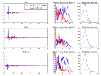
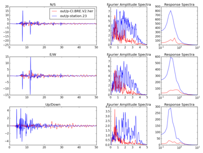
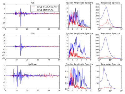
The plots below show La Habra observations compared to synthetic seismograms generated by Hercules for the following stations: FUL, BRE, DLA. The following parameters were used:
- gof.py
== Enter the sequence of sample rates: 0.15 0.25 0.5 1 2 4
== Enter the maximum frequence for decimation: 5
== Enter common dt of two signals: 0.025
== Enter azimuth for rotation (optional): 39.9
== Enter the earthquake start time (#:#:#.#): 4:9:42.97
== Enter the simulation leading time (sec): 0
- s_compare:
== Enter T-min for ploting: 0
== Enter T-max for ploting: 50
== Enter F-min for ploting: 0
== Enter F-max for ploting: 5
== Do you want to filter the data (y/n): n
== Enter tmin for Response: 0
== Enter tmax for Response: 10
== Do you want to cut the signal (y/n): n
- FUL
- BRE
- DLA
